Moderne Physik mit Maple
PDF-Buch Moderne Physik mit Maple
Update auf Maple 14 (Juli 2010)
Kapitel 3.3
Worksheet wellen3.mws
c International Thomson Publishing Bonn 1995 filename: wellen3.ms
Autor: Komma Datum: 6.11.93
Index: Wellen, Überlagerung
Thema: Form aus Kohärenz, Huygens Physik
Form aus Kohärenz
Vom mathematischen Standpunkt aus betrachtet, spielt die (od. eine) Wellengleichung für Wellen die gleiche Rolle wie die Newtonsche Gleichung für ein Teilchen: beides sind Bewegungsgleichungen -- als DGn formuliert. Aber es gibt einen entscheidenden Unterschied. Abgesehen davon, daß die WG nicht die Bewegung EINES Punktes beschreibt, läßt sie die lineare Superposition von Lösungen zu, was im Newtonschen Fall nur für die Schwingung möglich ist (oder ähnliche Kraftgesetze).
Diese Superpositionsfähigkeit -- und nicht die Beschreibung einer gleichförmigen Bewegung von ETWAS -- ist das entscheidende Charakteristikum des Phänomens Welle (Schwingung). Weil die Wellengleichung ohne Kraftgesetz auskommt, zählt nur das WIE der Bewegung und nicht das WAS oder WARUM. Und bei dem WIE interessiert nicht "wie schnell" und "wohin", sondern eben nur "auf welche Art". Superposition heißt: eine Welle kommt nie allein -- in Reinkultur. Selbst wenn man meint, man hätte genau eine einzige Welle vor sich, z.B. eine ebene Welle, so irrt man: diese einzige Welle läßt sich *zerlegen* in unendlich viele Wellen, und das auf viele verschiedene Arten. Das ist die Huygensche Physik: Wellen sind das *Ergebnis* von Superposition, Wellen interferieren. Wir wollen uns diesen Vorgang zunächst in der räumlichen Darstellung veranschaulichen und in einem weiteren Abschnitt auf die Details der wichtigen Sonderfälle wie Doppelspalt, Gitter und Spalt zurückkommen. Das ist typisch für das Vorgehen mit einem CAS: im Gegensatz zu herkömmlichen Methoden, die meist vom Einfachen, Elementaren zum Komplexen führen, kann mit einem CAS ein komplexer Zusammenhang direkt angegangen werden, zumindest was seine Veranschaulichung betrifft. Und dann kann weiter analysiert und zerlegt werden.
Nach Huygens kann jeder Punkt einer Wellenfront als Zentrum einer Elementarwelle aufgefaßt werden.
Wir versuchen, eine nach oben laufende Welle mit geraden Fronten zunächst mit Zentren zu erzeugen, die auf einer Geraden liegen, also z.B. durch Kreiswellen in der x-y-Ebene mit Zentren auf der x-Achse
| > |
| (1) |
| > |
| (2) |
| > |
| (3) |
| > |
| (4) |
| > |
| (5) |
| > | for j to n do |
| > | x0[j]:=2*j od: |
| > |
| (6) |
| > |
Animation der Wellenfronten
| > |
| (7) |
| > |
| (8) |
| > |
|
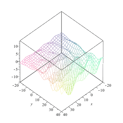
Dreidimensionale Animation
| > |
| (9) |
| > |
|
Die Wellenfronten sind je nach Anzahl und Dichte der Zentren im Nahbereich "gerade" und aus großem Abstand sieht ohnehin alles wie ein Punkt aus und sendet somit Kugelwellen. Aber unsere Konstruktion hat einen Nachteil: die Welle läuft in zwei Richtungen. Man hört ja auch manchmal die Scherzfrage, ob sich Huygens nicht geirrt habe -- denn wie kann aus Wellen die in alle Richtungen laufen, eine geordnete Bewegung in eine Richtung entstehen?
Untersuchen wir also, ob sich Huygens geirrt hat. Dazu müssen wir die Anordnung unserer Zentren in die Ebene ausdehnen.
Array von regelmäßig angeordneten Zentren
| > |
| (10) |
| > |
| (11) |
| > |
| (12) |
| > |
| (13) |
| > |
| (14) |
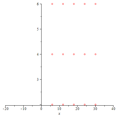
| > | for ii to n do |
| > | for jj to m do |
| > |
| > | y0[ii][jj]:=2*jj od: od: |
| > |
|
winpl():
| > |
| (15) |
| > |
| (16) |
| > |
| (17) |
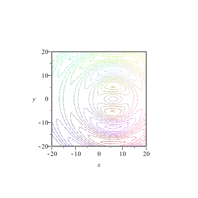
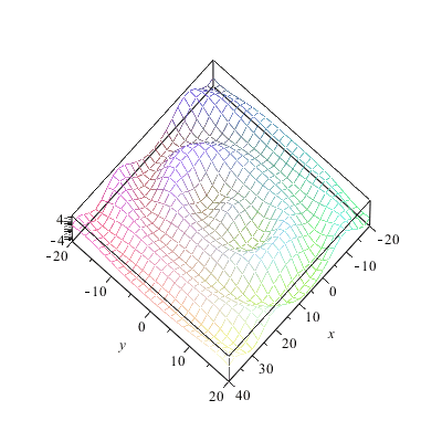
| > | wani3:=animate3d(welle,x=-20..40,y=-20..40,t=0..2*(1-1/nf)*Pi/w,axes=boxed,style=contour, |
| > | scaling=constrained,orientation=[-90,0],frames =nf): |
| > |
|
| > |
|
| > |
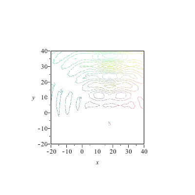
Jetzt läuft schon wesentlich mehr nach oben als nach unten.Woran liegt das? An der regelmäßigen Anordnung der Zentren? Daran liegt es auch (man kann die Zentren aber auch "schlecht" anordnen, probieren Sie doch mal Ihre eigene Anordnung aus). Aber an der Anordnung der Zentren liegt es nicht in erster Linie, wie folgender Versuch beweist:
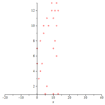
Lage der Zentren zufallsverteilt
| > |
| (18) |
| > |
| (19) |
| > | for ii to n do |
| > | for jj to m do |
| > |
| > | y0[ii][jj]:=zuf() od: od: |
| > |
|
| > |
| (20) |
| > |
|
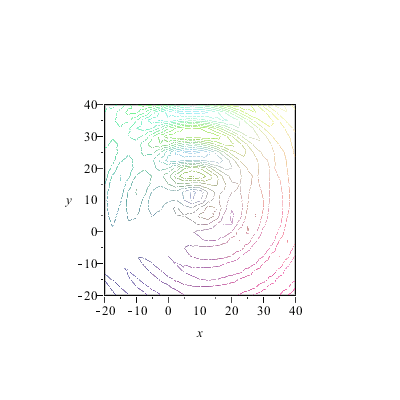
*Wo* die Zentren liegen spielt also keine entscheidende Rolle für die Form der Wellenfronten und ihre Ausbreitungsrichtung, solange es nur genügend viele Zentren sind. Es kommt vielmehr auf die "richtige" Phasenbeziehung an (die natürlich oben in die Formeln hineingesteckt wurde). Und Huygens hat also recht, wenn er sagt, daß JEDER Punkt einer Wellenfront als Zentrum einer Elementarwelle aufgefaßt werden kann. Aufgefaßt? Es *ist* so, daß die Phasenbeziehung und damit die Kohärenz die Form bestimmt.
Wir wollen uns das an einem eindimensionalen Schnitt in y-Richtung veranschaulichen, d.h. wir setzen nun Zentren auf die y-Achse, "steuern sie mit der richtigen Phase an", addieren die Amplituden der in beide Richtungen laufenden Wellen und verfolgen ihre Ausbreitung.
| > |
| (21) |
| > |
| (22) |
| > |
| (23) |
| > |
| (24) |
| > |
| (25) |
| > | for j to n do |
| > | y0[j]:=Pi/k*j/n od: |
| > |
| (26) |
| > |
| (27) |
| > |
| (28) |
| > |
|
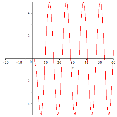
Es funktioniert! Aber wo sind die Wellen auf der negativen y-Achse geblieben? Haben wir das auch richtig programmiert? Eine Kontrolle wäre wohl angebracht:
| > |
| (29) |
| > |
|
| > |
| (30) |
| > |
|
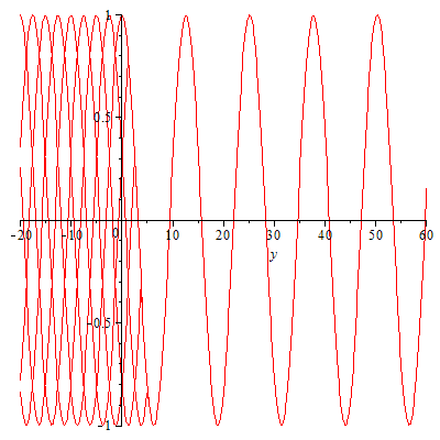
Alle Elementarwellen sind da! Aber die nach links laufenden können sich nicht einigen und löschen sich gegenseitig aus: Wellensalat! Studieren Sie auch das Übergangsgebiet, also das Gebiet, in das Sie Zentren setzen (was kann man alles ändern?).
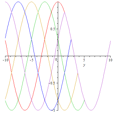
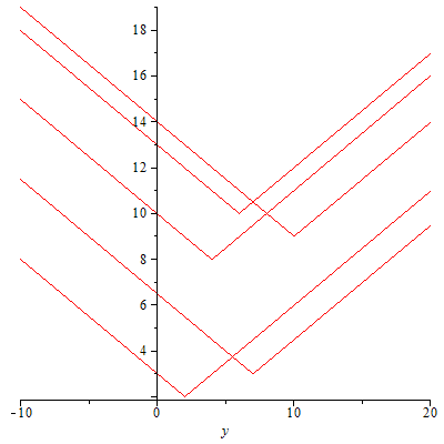
Man kann den Sachverhalt "Verstärkung in Vorwärtsrichtung -- Auslöschung in Rückwärtsrichtung" auch noch etwas anders darstellen, allerdings etwas abstrakter, indem man sich die Phasen der Elementarwellen über dem Ort darstellen läßt.
| > |
| (31) |
| > |
| (32) |
| > |
| (33) |
| > |
| (34) |
| > |
| (35) |
| > |
|
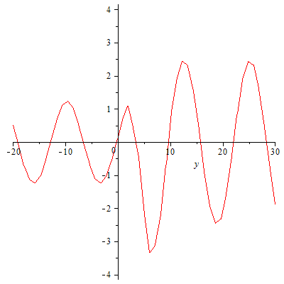
Für inkohärente Elementarwellen hätte man dagegen
| > |
| (36) |
| > |
| (37) |
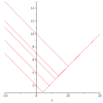
Die "Charakteristiken" wären beliebig verteilt
| > |
|
| > |
| > |
| (38) |
Und eine geordnete Bewegung könnte nur zufällig zustandekommen
| > |
| (39) |
| > |
|
Siehe auch: Kohärenz durch Ausbreitung | Gitter | Fresnelbeugung | Zeiger | Photon am Doppelspalt | Kohärenzlänge
komma(AT)oe.uni-tuebingen.de